Making Your Research Reproducible with R

Post provided by Laura Graham

Reproducible research is important for three main reasons. Firstly, it makes it much easier to revisit a project a few months down the line, for example when making revisions to a paper which has been through peer review.

Secondly, it allows the reader of a published article to scrutinise your results more easily – meaning it is easier to show their validity. For this reason, some journals and reviewers are starting to ask authors to provide their code.

Thirdly, having clean and reproducible code available can encourage greater uptake of new methods. It’s much easier for users to replicate, apply and improve on methods if the code is reproducible and widely available

Throughout my PhD and Postdoctoral research, I have aimed to ensure that I use a reproducible workflow and this generally saves me time and helps to avoid errors. Along the way I’ve learned a lot through the advice of others, and trial and error. In this post I have set out a guide to creating a reproducible workflow and provided some useful tips.

Setting Up a Workflow

My first step in setting up a reproducible workflow in R is to begin a new project in RStudio. R projects enable you to “divide work up into multiple contexts, each with their own working directory, workspace, history, and source documents”. Basically, this means that each R project is self contained, which allows for greater portability of projects – great for if you are working with collaborators or across more than one computer. Also, because the workspace and open source files are saved separately for each project, the R projects framework allows users to switch between projects and just pick up where they left off – perfect for multi-taskers!

Next is version control. Version control allows you to keep track of how a project evolves, to create new ‘branches’ for testing out changes to code, and to revert to previous versions if anything goes wrong. Git works nicely alongside RStudio, and there is plenty of support online for using this version control system. It links into GitHub, which is a repository hosting service that makes collaboration much easier by acting as a central point for a project.

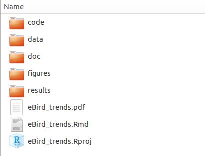
Finally, I find that having an effective folder management system which works for me makes all the difference in the initial project set up. Here’s my folder set up:

This works well for me, but may not be optimal for everyone. Experiment with different structures and find what’s best for you!

Additional tips for setting up a reproducible workflow are to annotate all code to explain the steps and reasoning behind them. Using relative file paths is also a good idea (data.csv rather than C:/ProjectFolder/data.csv) as it makes code more portable, and the R project has already set the project directory for you!

Loading Data

R can handle data from a lot of different sources. readr tends to work faster than base R for flat files (.csv, .txt), so is particularly useful if you’re reading in huge amounts of data. readxl can read Excel spreadsheets into R, RODBC works for many types of databases (including Microsoft Access), and RPostgreSQL interfaces with PostgreSQL databases. A new package now allows for interacting with googlesheets too. It is also possible to load spatial data in R using the raster and rgdal packages. Generally, if you have data in a reasonably widely used format, someone has probably written a package to read it into R.

Data Tidying and Manipulation Tools

“Tidy datasets are all alike but every messy datset is messy in its own way” (Hadley Wickham, 2014)

Key features of tidy data are:

• Observations in rows
• Variables in columns
• Each type of observational unit is a table

Messy data can take many forms. For example:

• Column headers are values, not variable names
• Multiple variables stored in one column
• Variables stored in both rows and columns
• Multiple observational unit types in the same table
• Single observational unit in multiple tables

Aspiring for tidy data makes data analysis much more straightforward, and this is made much easier with the use of a set of R packages. tidyr provides tools for tidying data frames and works well with dplyr, which contains tools for fast data manipulation. lubridate makes dealing with dates much easier and taxize provides functionality for working with taxonomic data, such as resolving taxonomic names. These packages are user friendly and will make things much simpler for you in the short- and long-term.

Dealing with Messy Output

Data analysis in R often leads to very messy output:

data("mtcars")
lmfit <- lm(mpg ~ wt, mtcars)
summary(lmfit)

## 
## Call:
## lm(formula = mpg ~ wt, data = mtcars)
## 
## Residuals:
##     Min      1Q  Median      3Q     Max 
## -4.5432 -2.3647 -0.1252  1.4096  6.8727 
## 
## Coefficients:
##             Estimate Std. Error t value Pr(>|t|)    
## (Intercept)  37.2851     1.8776  19.858  < 2e-16 ***
## wt           -5.3445     0.5591  -9.559 1.29e-10 ***
## ---
## Signif. codes:  0 '***' 0.001 '**' 0.01 '*' 0.05 '.' 0.1 ' ' 1
## 
## Residual standard error: 3.046 on 30 degrees of freedom
## Multiple R-squared:  0.7528, Adjusted R-squared:  0.7446 
## F-statistic: 91.38 on 1 and 30 DF,  p-value: 1.294e-10

While this summary is useful for assessing the output of a single model, it can become quite difficult once the number of models starts to increase. This is where the broom package comes in handy. This package provides functions to convert model coefficient estimates, predicted values and residuals, and summary statistics to data frames.

library(broom)
tidy(lmfit)

##          term  estimate std.error statistic      p.value
## 1 (Intercept) 37.285126  1.877627 19.857575 8.241799e-19
## 2          wt -5.344472  0.559101 -9.559044 1.293959e-10

glance(lmfit)

##   r.squared adj.r.squared    sigma statistic      p.value df    logLik
## 1 0.7528328     0.7445939 3.045882  91.37533 1.293959e-10  2 -80.01471
##        AIC      BIC deviance df.residual
## 1 166.0294 170.4266 278.3219          30

Plotting

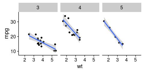
ggplot2 is designed to work with tidy data formats and is based on the idea of the grammar of graphics. This concept makes building up graphs from very simple to complex quite straightforward by adding additional layers. However, ggplot2 does have some less than ideal formatting like a grey gridded background. The cowplot package overrides some of these settings to make publication quality plots. Cowplot also has some nice functionality for arralibrary(ggplot2)

library(ggplot2)
library(cowplot)
ggplot(mtcars, aes(x = wt, y = mpg)) + 
  geom_point() + 
  facet_wrap(~gear) + 
  geom_smooth(method = "lm")

RMarkdown

Finally, all analyses can be combined into a literate format using RMarkdown. RMarkdown combines the Markdown markup language, knitR (which facilitates the inclusion of R code chunks) and pandoc (which converts markdown to a range of formats including PDF, word, HTML and notebooks). Using RMarkdown allows you to keep a dynamic log of analysis and the syntax is reasonably simple (with a lot of online resources available to help!).

Additional Resources

I hope that you’ve found this guide to making your research more reproducible with R helpful. If you’d like to learn more about R or about reproducibility, I’d highly recommend the following resources:

• RStudio cheatsheets: includes ggplot2, RMarkdown, dplyr, tidyr and more
• Swirl: tutorials for tidyr, dplyr and much more directly in the R console
• Python pandas comparison with R: a more detailed look at the R language and its many third party libraries as they relate to pandas
• Software Carpentry lessons: freely available lessons taught on the Software Carpentry courses. To host or run a workshop also see this site.
• Reproducible Research on Coursera: taught by Roger Peng, Jeff Leek and Brian Caffo at Johns Hopkins University
  

  ---

 Workshop: Best Practice for Code Archiving
12:00 – 17:00 Sunday 11 December
Price: £10

Interested in how to distribute and archive code? Join Methods in Ecology and Evolution Editors Rob Freckleton and Bob O’Hara and as well as several experts with backgrounds in programming and ecology for a practical discussion of writing and sharing code for your research at the BES Annual Meeting. All levels of expertise are welcome, especially those just starting out.

---